Heat Transfer

Heat transfer is an important topic in many engineering cases. Heat transfer describes heat flows inside a material or between materials. It can be divided into three main categories conduction, convection and thermal radiation. In the following each will be dealt with from a practical point of view including examples on how to calculate heat transfer in different cases.

Conduction - Fourier's Law

Conduction also known as Thermal Conduction is the transfer of internal energy within a material. The energy is transferred by collision of molecules, atoms and electrons inside the material. The heat flow will occur in solid, liquid and plasma phases and the energy will always flow from hot to cold.

Joseph Fourier created Fourier's Law also known as The Law of Heat Conduction which defines heat transfer or heat flow through a solid object.

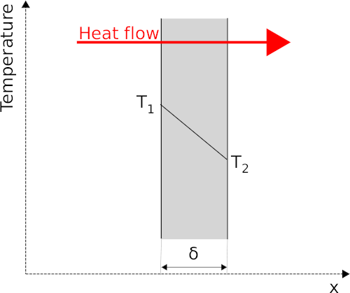
For heat conduction through a one-dimensional solid plane the equation is:

\begin{align} q=-\lambda \frac{dt}{dx} \end{align}

where:

q is the heat flow per unit area [W/m²]
λ is the thermal conductivity [W/(m K)]
dt/dx is the temperature gradient [K/m]

The equation is valid for heat transfer in one-direction (x) perpendicular to the surface from hot to cold. Heat do however not only transfer in one-direction. In the following however it will be assumed that the temperature is stationary i.e. is not changing with time and that the conduction is one-dimensional. This is of-course not always the case but it is valid for in many cases.

The heat flow from the hot side of the plane T₁ to the cold side T₂ for the entire plane is:

\begin{align} \Phi = \frac{\lambda }{\delta }A(T_1 - T_2) \end{align}

where:

Φ is the heat flow [W]
δ is wall thickness [m]
A is surface area [m²]
λ is the thermal conductivity [W/(m K)]
T₁ plane surface temperature hot side [K]
T₂ plane surface temperature cold side [K]

Thermal Conductivity

Thermal conductivity λ is the ability of a material to conduct heat. The material constant is temperature dependent and the mean temperature is used for table lookup unless other is noted i.e. \( \frac{T_1+T_2}{2} \). The value is typically largest for heavy materials i.e. heavy materials conduct heat better and lower for light materials. For absolute vacuum for example the thermal conductivity is zero as no conduction is possible. The value typically declines with increasing temperature for metals and increases with increasing temperature for gasses i.e. cold metals conduct better than hot metals and hot gasses conduct better than cold gasses.

Various λ values are collected in the table below.

Table 1 - Thermal conductivity for various solid materials
Material	Thermal conductivity λ [W/(m K)]
Aluminum	229
Boiler steel H III	52
Brass	95
Bronze	61.7
Cast iron 3% C	58
Cobber pure	395
Cobber typical	372
Crome-nickel steel	14.5
Lead	35.1
Iron	59
Gold	310
Magnesium pure	143
Nickel	60-90
Silver	410
Zinc	113
Tin	66
Platinum	70

Thermal Resistance - multiple layers with different properties

Often a wall, ceiling etc. consist of more than one material. Is is because of this necessary to look into how to treat planes with multiple layers of different materials and different thicknesses.

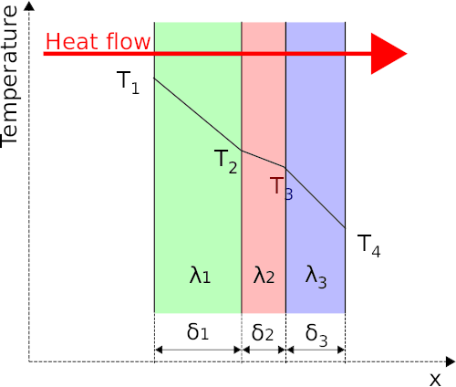
Thermal conduction through a 3 layered wall

The solution is to determine a combined thermal resistance similar to electrical resistances in serial using Ohms Law. The thermal resistance in the system shown in the figure above will be determined using Fourier's law. The wall consist of 3 layers each with different thermal conductivity and layer thickness. The total heat flow through all of the layers Φ will also flow through each independent layers hence:

\begin{align} \Phi = \frac{\lambda _1 }{\delta _1}A(T_1 - T_2) = \frac{\lambda _2 }{\delta _2}A(T_2 - T_3) = \frac{\lambda _3 }{\delta _3}A(T_3 - T_4) \end{align}

This is equivalent to resistors in seria similar to Ohms law hence the total thermal resistance can be written as:

\begin{align} R_{tot} = R_1+R_2+R_3 = \frac{\delta _1}{\lambda _1 A}+\frac{\delta _2}{\lambda _2 A}+\frac{\delta _3}{\lambda _3 A} \end{align}

The equation for thermal resistance can be expanded to as many layers as needed.

Adding this to Fourier's Law gives

\begin{align} \Phi = \frac{1}{R}(T_1-T_4) \end{align}

where

Φ is the heat flow [W]
R is the absolute thermal resistance for all layers [K/W]
T₁ plane surface temperature hot side [K]
T₄ plane surface temperature cold side [K]

Cylindrical Wall i.e. pipes and similar

The procedure above for a plane can be used for thin walled cylinders and cylinders with large diameters. The case is however different for cylinders with large wall thickness e.g. an insulated pipe as the heat flow will not be one-directional as assumed for the plane.

Using Fourier's law one can determine that for a single layer thick walled cylinder the heat flow is:

\begin{align} \Phi = \frac{\lambda 2 \pi L(T_1-T_2)}{ln\frac{r_2}{r_1}} \end{align}

where:

Φ is the heat flow [W]
L is the length of the cylinder [m]
λ is the thermal conductivity [W/(m K)]
T₁ plane surface temperature hot side [K]
T₂ plane surface temperature cold side [K]
r₁ inner radius of the cylinder [m]
r₂ outer radius of the cylinder [m]

The thermal resistance R [K/W] can now for a single layer be determined as:

\begin{align} R = \frac{T_1-T_2}{\Phi } = \frac{ln\frac{r_2}{r_1}}{\lambda 2 \pi L} \end{align}

The thermal resistance is used the same way as for the plane described in the previous section.

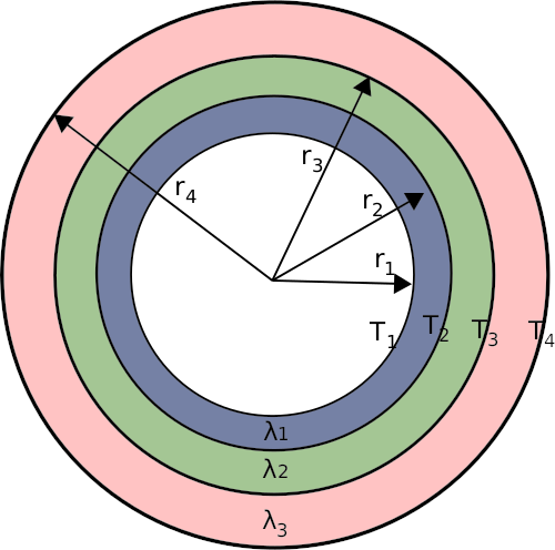
Similar to the approach used for the 3-layered plane it can be expanded to several layers with different properties. For the 3-layered cylinder seen on the figure above the thermal resistance is:

\begin{align} R_{tot} = R_1+R_2+R_3 = \frac{1}{2\pi L}\left( \frac{1}{\lambda _1}ln\frac{r_2}{r_1}+\frac{1}{\lambda _2}ln\frac{r_3}{r_2}+\frac{1}{\lambda _3}ln\frac{r_4}{r_3} \right) \end{align}

And similar to the plane case the heat flow can be determined:

\begin{align} \Phi = \frac{1}{R_{tot}}(T_1-T_4) \end{align}

The two equations above is for 3 layers but can be expanded to as many layers as needed.

Convection

Convection also known as convective heat transfer is heat moved by the movement of gasses or liquids. Two types exist, i.e. forced and natural convection. Natural convection is when the fluid movement is created by buoyancy forces due to changes in fluid density.

One example is heating water in a pot. The water is heated at the bottom hence the water at the bottom gets hotter and the hot water will start to rise and the cold will sink. The reason for this is that water density will change with changing temperature.

Another example is the creation of cumulus clouds. When rays from the sun a surface it will be heated. Some surfaces will get hotter than others e.g. tarmac and sand whereas water and trees will not be heated less. Air density decreases with increasing temperature hence the hot air will start to rise and will bring hot and moist air upwards. This is convection. The air pressure is decreasing with altitude leading to hot air getting colder and at some height equilibrium between the rising and surrounding air is obtained. If the air temperature gets below the dew point a cumulus cloud will be formed. This is however an completely different topic that I at some point in time will cover in a separate article.

The other type of convection Forced Convection is created by forced flows over the surface. Examples are fluid pumped through a pipe, ventilator forcing air along a surface, wind outside etc.

It is however not uncommon that both appear at the same time. This is sometimes called mixed convection.

Determining the heat transfer from convection requires model equations making it possible to determine the Nusselt Number for the specific use case.

Newtons Equation

Heat flow from a fluid to a surface or vice versa can be determined by Newtons equation. Determination of the Convection heat transfer coefficient α (sometimes denoted with the letter h instead of α) requires calculation of the Nusselt Number as described in the following sections.

\begin{align} \Phi = \alpha A(T_{fluid}-T_{surface}) \end{align}

where:

α Convection heat transfer coefficient [W/(m²K)]
A Surface area [m²]
T_fluid Fluid temperature [K]
T_surface Surface temperature [K]

Nusselt Number

The Nusselt Number named after Wilhelm Nusselt, who made a large contribution to the science of convection, is a dimensionless coefficient which describes the ratio between convective and conductive heat transfer at a plane or wall.

\begin{align} Nu_L=\frac{\text{Convective heat transfer}}{\text{Conductive heat transfer}} = \frac{\alpha }{\lambda /L} = \frac{\alpha L}{\lambda } \end{align}

where:

α Convection heat transfer coefficient [W/(m²K)]
λ Thermal conductivity [W/(m K)]
L is the characteristic length

Determination of the Nusselt Number depends upon the case. For free convection the average Nusselt number is a function Rayleigh number and Prandtl number and in case of forced convection it is a function of Reynolds Number and Prandtl number.

Reynolds number

Reynolds number is the ratio between inertial to the viscous forces hence it can be used to describe the flow type.

\begin{align} Re = \frac{cL}{\nu } \end{align}

where:

c Flow velocity [m/s]
L Characteristic length [m]
ν Kinematic viscosity [m²/s]

Grashof Number

Dimensionless ratio between buoyancy to viscous forces

\begin{align} Gr = \frac{gL^3\alpha _v \Delta T}{\nu ^2} \end{align}

where:

g Gravitational acceleration 9.81m/s²
L Characteristic length [m]
\( \alpha _v \) Thermal expansion coefficient [1/K]
\( \Delta T \) Temperature difference [K]
ν Kinematic viscosity [m²/s]

Prandtl Number

Prandtl number also known as Prandtl group is a dimensionless material constant defining the ratio of momentum diffusivity to thermal diffusivity. Can be found in various tables and by use of property calculators including the ones on this website e.g. the water property calculator and the steam property calculator.

\begin{align} Pr = \frac{\eta c_p}{\lambda } \end{align}

where:

η dynamic viscosity [Pa×s]
c_p Specific isobaric heat capacity [J/(kg×K)]
λ Thermal conductivity [W/(m×K)]

Rayleigh Number

Rayleigh number is a dimensionless number based on Grashoff number and Prandtl number. It is used in cases with free convection to characterise the flow regime.

\begin{align} Ra = Gr Pr \end{align}

Procedure to determine the convection heat transfer coefficient

Determine the geometry and flow type. Make a drawing
Determine reference temperature as defined by the equations matching the geometry and flow type. This is however often the film temperature i.e. \( T_{film}=\frac{T_{fluid}-T_{wall}}{2}\) but it can also be the fluid temperature \( T_{fluid} \)
Calculate Reynolds number in case of forced convection and determine if the flow is laminar or turbulent and calculate Prandtl number
Select model equation based on the above
Calculate Nusselt number
Calculate convection heat transfer coefficient

Forced Convection

The Nusselt number is for forced convection a function of Reynolds number and Prandtl number.

Flow along a plane

The convection heat transfer coefficient will change along the plane as the flow type changes. The flow will start as laminar but can change to turbulent flow if the plate is long enough and the flow velocity high enough. The location for the change depends upon the plate shape and velocity but normally the critical value of Reynolds number is 5×10⁵.

The characteristic length L is the plate length along the flow direction.

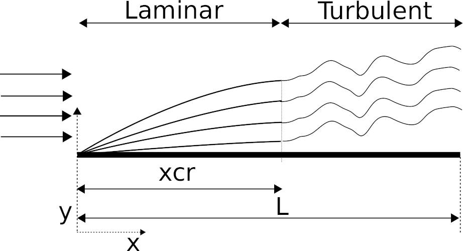
Reynolds number < 5×10⁵ - Laminar flow

The Nusselt number is for the laminar flow over the entire length (L) of the plane i.e. Reynolds number below 5×10⁵ calculated as:

\begin{align} Nu_m = 0.664Re_m^{0.50}Pr^{1/3} \end{align}

Thermodynamic properties to be determined at film temperature i.e. \( T_{film}=\frac{T_{fluid}-T_{wall}}{2} \)
Valid for 0.6<Pr<50
Characteristic length L is the plate length in the flow direction [m]

Reynolds number > 5×10⁵ - Turbulent flow

The Nusselt number is for the turbulent flow calculated as below. The equation includes the effect that the first part of the flow will be laminar and the last turbulent hence it shall not be divided into a laminar and a turbulent part but can be treated as one.

\begin{align} Nu_m = \left( 0.037Re^{4/5}-871 \right) Pr^{1/3} \end{align}

Thermodynamic properties to be determined at film temperature i.e. \( T_{film}=\frac{T_{fluid}-T_{wall}}{2}\)
Valid for 0.6<Pr<50
Characteristic length L is the plate length

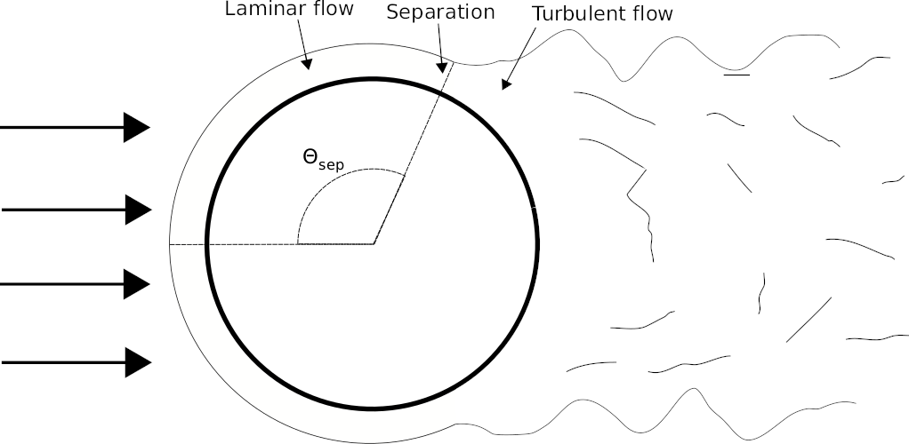
Flow across a cylinder

The Nusselt number is for external flow across a cylinder (See sketch below) determined using:

\begin{align} Nu_m = C Re^m Pr^n \left( \frac{Pr}{Pr_v} \right) ^{1/4} \end{align}

Valid for 0.7<Pr<50 and 1<Re<10⁶
Thermodynamic properties to be determined at fluid temperature
n=0.37 for Pr<=10
n=0.36 for Pr>10
The characteristic length is the diameter
The constant C and m depends upon the Reynolds number and can be found using the table below

Forced convection. Flow around a cylinder showing laminar flow, separation angle and turbulent flow.

Table 1 - Coefficient used to determine the Nusselt number for flow across a cylinder
Reynolds number - Re	C	m
1 - 40	0.75	0.4
40 - 1000	0.51	0.5
1000 - 2×10⁵	0.26	0.6
2×10⁵ - 10⁶	0.076	0.7

Forced internal flow

Forced internal flow i.e. flow in ducts and pipes are contrary to forced external flow not able to develop freely due to the interference from the internal surface. It is as a consequence of this necessary to look at the pipe/duct upstream of the section to fully understand the flow. The length of this upstream section that has to be considered is typically calculated as:

\begin{align} & \frac{x_{inlet}{D} = 0.05Re \text{ Laminar flow}\\ & 10<\frac{x_{inlet}}{D}<60 \text{Turbulent flow} \end{align}

where:

D is the diameter or hydraulic diameter in case of non-circular pipes/ducts [m]
Re is the Reynolds number
x_inlet is the length of the inlet section to be considered

Laminar flow - Re<2300

The Nusselt number is for laminar flow i.e. Reynolds number below 2300 calculated as:

\begin{align} Nu_m = 3.66+\frac{0.0668\frac{D}{L}RePr}{1+0.04\left( \frac{D}{L}RePr\right)^{2/3}} \end{align}

where:

L is the length of the pipe [m]
D is the diameter or hydraulic diameter in case of non-circular pipes/ducts [m]
Re is the Reynolds Number
Pr is the Prandtls Number

Turbulent flow - Re>2300

In case of turbulent flow i.e. Reynolds number above 2300 the Nusselt number is:

\begin{align} Nu_m = 0.0235\left( Re^{0.8}-230 \right) \left( 1.8Pr^{0.3}-0.8\right) \left( \frac{\eta}{\eta _w}\right) ^{0.14} \left( 1+\left( \frac{D}{L}\right) ^{2/3} \right) \end{align}

where

L is the length of the pipe [m]
D is the diameter or hydraulic diameter in case of non-circular pipes/ducts [m]
Re is the Reynolds Number
Pr is the Prandtls Number
η dynamic viscosity at fluid mean temperature [Pa×s]
η_w dynamic viscosity at wall surface temperature [Pa×s]

Free Convection

The flow driven by free convection is contrary to forced convection not created by pumps, fans etc. but is instead created by thermal forces happening because of density gradient in the fluid.

The Rayleigh number is used to determine the flow type in a similar manner as Reynolds number was used for forced convection to determine whether the flow is laminar or turbulent.

\begin{align} Ra=Gr Pr =\frac{g\alpha _v (T_w-T_{fl})L^3}{\nu a} \end{align}

where:

\begin{align} a= \frac{\lambda }{c_p \rho } \end{align}

g Gravitational acceleration 9.81m/s²
L Characteristic length [m]
α_v Thermal expansion coefficient [1/K]
ν Kinematic viscosity [m²/s]
T_w Surface temperature [K]
T_fl Fluid temperature [K]
λ Thermal conductivity [W/(m K)]
c_p Specific isobaric heat capacity [kJ/(kg×K)]
ρ Density [kg/m³]

External free convection

Free convection can in case of plane surfaces be calculated using the equation below. The constant C depends upon the actual case as described in the following sections.

\begin{align} Nu_m = C Ra_L^n \end{align}

where:

L is the characteristic length
n = 1/4 for laminar flow
n = 1/3 for turbulent flow i.e. \( Ra>Ra_{kr}=10^9\)
Thermodynamic properties determined at film temperature
C is depend upon the actual case

Vertical plane

The constant C is in case of a vertical plane as follows. Notice that the plane is not divided into a laminar and turbulent part in case of turbulent flow on part of the plane.

C=0.59 with laminar flow
C=0.10 with turbulent flow. This value is then used for the entire length including the laminar part
L the characteristic length is the height H

Horizontal plane

Flow upwards from heated surface or downwards from cooled surface

C = 0.54 Laminar flow
C = 0.15 Turbulent flow
The characteristic length L is the surface area divided by the circumference

Flow down on heated surface or up onto a cooled surface - C = 0.27 for laminar and turbulent flow

Horizontal cylinder

The Nusselt number is for a horizontal cylinder such as a heating/cooling pipe determined by;

\begin{align} Nu_m = \left( 0.6+\frac{0.387Ra^{1/6}}{(1+(0.559/Pr)^{9/16})^{8/27}} \right) ^2 \end{align}

Valid for 10^-5<Ra<10¹²
The characteristic length is the diameter
Thermodynamic properties to be determined at film temperature

Radiation

Convection is not the only heat flow from a surface as thermal radiation will radiate energy as electromagnetical waves at the speed of light. The percentage of the entire heat flow due to thermal radiation increases with temperature and consequently gets more important at higher surface temperatures. The contribution can in some cases be omitted if the surface temperature is low as convection will contribute with the largest amount of heat flow.

Thermal radiation energy from electromagnetical waves will when hitting an object either be:

Reflected similar to a mirror. The spectral reflection component r.
Absorbed. The spectral absorption component a.
Passed through the object. The spectral transmission component d.

Non of the energy is lost hence the three component added together equals one.

\begin{align} r + a + d = 1 \end{align}

Perfect black materials (this is not referring to the color) absorb all of the thermal radiation hence a=1. For perfect white materials (again not referring to the color) all of thermal radiation hitting to surface will be reflected hence r=1. All other materials are called grey and will have a<1 and r<1.

Kirchoff's Law - Emissivity Coefficient

All objects that absorb thermal radiation will also emit thermal radiation also called emission. Gustav Kirchoff determined that the emitted thermal radiation equals the absorbed thermal radiation. This is known as Kirchoff's Law and can be written as the absorption component a equals the emissivity coefficient ε.

\begin{align} \epsilon = a \end{align}

where:

ε is the emissivity coefficient
a is the spectral absorption component

The table below contains emissivity coefficients for various selected materials.

BESKRIV n og h i tabel

Table X - Emissivity Coefficient for selected materials
Material	Emissivity Coefficient ε
Skin (h)	0,95
Asbestos grey (h)	0.96
Cobber polished (h) 600K	0.04
Stainless Steel polished (n) 600K	0.19

Stefan-Boltzmann's Law

Thermal radiation is calculated using the Stefan-Boltzmann's Law. It states that for a perfect black object the thermal radiation in W/m² equals:

\begin{align} E_s = \sigma T^4 \end{align}

Where σ is the Stefan-Boltzmann constant and T is the surface temperature in Kelvin.

\begin{align} \sigma = 5.67\cdot 10^{-8} \frac{W}{m^2K^4} \end{align}

The equation is often written as

\begin{align} E_s = C_s\left( \frac{T}{100} \right) ^4 \end{align}

where the constant C_s equals

\begin{align} C_s = 10^8 \sigma =5.67W/(m^2 K^4) \end{align}

For non-black objects called grey objects the emissivity coefficient ε is used

\begin{align} E=\epsilon E_s = \epsilon \sigma T^4=\epsilon C_s\left( \frac{T}{100} \right) ^4 \end{align}

Lambert's Cosine Law

Thermal radiation is emitted in all directions i.e. not only perpendicular to the surface. Lambert's Cosine Law also known as the Cosine Emission Law or Lambert's Emission Law makes it possible to determine the radiation intensity emitted at any angle to the surface.

\begin{align} E_{\phi } = E_n\cdot cos\phi \end{align}

where φ is the angle from perpendicular to the surface i.e. φ=0deg when radiation emitted perpendicular to the surface and φ=90deg along the surface.

The correlation between the total radiated intensity E and the intensity normal to the surface E_n can by using the equation above be found to be:

\begin{align} E =\pi E_n \end{align}

Thermal Radiation between Surfaces

Two surfaces with different temperatures placed opposite of each other will exchange heat to each other by thermal radiation. The heat radiated from the hot surface will be higher than the heat radiated by the cold. The direction of the heat flow will therefore be from the hot surface (surface 1) to the cold surface (surface 2).

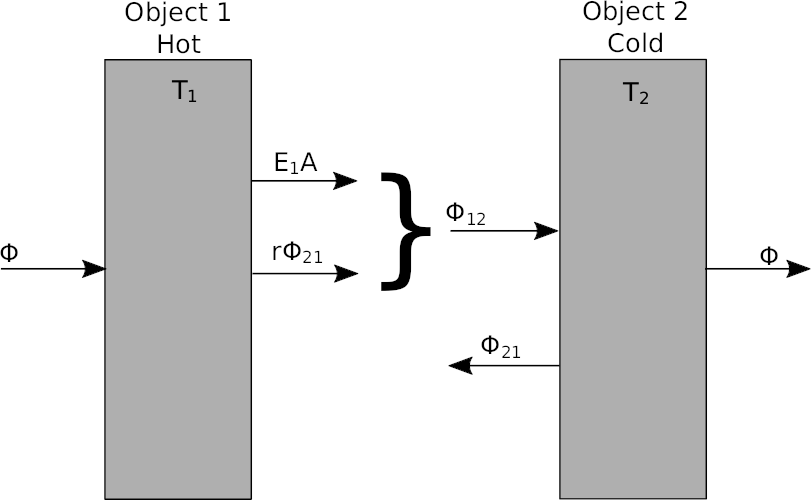
Both surfaces will radiate heat and both surfaces will also reflect some of the heat as none of the surfaces are perfect black or white. It is in this example assumed that no thermal radiation escapes the other surface hence no energy is lost to the surroundings.

Φ₁₂ total thermal energy radiated from surface 1 towards surface 2 including reflected thermal energy.
Φ₂₁ total thermal energy radiated from surface 2 towards surface 1 including reflected thermal energy.

\begin{align} \Phi _{12} &=E_1A+r_1\Phi _{21} \\ \Phi _{21} &=E_2A+r_2\Phi _{12} \end{align}

where:

E₁ and E₂ thermal radiation from surface 1 and 2 respectively [W/m²]
r₁ and r₂ spectral reflection component for surface 1 and 2 respectivly
A, Surface area. The areas are in this example identical[m²]

The total heat flow from surface 1 (hot surface) to surface 2 (cold surface) is:

\begin{align} \Phi = \Phi _{12}-\Phi _{21} \end{align}

Combining this together with the equation for thermal radiation determined in previous sections \( E=\epsilon \sigma T^4=\epsilon C_s\left( \frac{T}{100} \right) ^4 \) and using that \( \epsilon=a \) as defined in Kirchoff's Law.

\begin{align} \Phi = \sigma _{12}A(T_1^4-T_2^4) \end{align}

or by using C instead of σ

\begin{align} \Phi = C_{12}A\left( \left( \frac{T_1}{100} \right) ^4 -\left( \frac{T_2}{100} \right) ^4 \right) \end{align}

where:

\begin{align} \sigma _{12}=\frac{\sigma }{\frac{1}{\epsilon _1}+\frac{1}{\epsilon _2}-1} \\ C_{12} =\frac{C_s }{\frac{1}{\epsilon _1}+\frac{1}{\epsilon _2}-1} \end{align}

ε₁ emissivity coefficient surface 1
ε₂ emissivity coefficient surface 2
σ the Stefan-Boltzmann constant \( 5.67\cdot 10^{-8} \frac{W}{m^2K^4} \)
C_s is \( C_s = 10^8 \sigma =5.67W/(m^2 K^4) \)
T₁ surface area hot side
T₂ surface area cold side

Object located inside a surrounding object

The solution will be very similar for this case where an object is located inside a surrounding object as the only difference is that the areas are not identical.

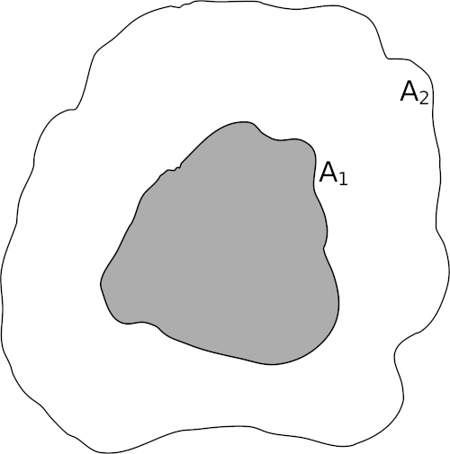
Object located inside a surronding object — Object located inside a surrounding object

\begin{align} \sigma _{12} &= \frac{\sigma }{\frac{1}{\epsilon _1}+\frac{A_1}{A_2}\left( \frac{1}{\epsilon _2}-1 \right) } \\ C _{12} &= \frac{C_s}{\frac{1}{\epsilon _1}+\frac{A_1}{A_2}\left( \frac{1}{\epsilon _2}-1 \right) } \end{align}

where A₁ and A₂ is the areas for surface 1 and 2 respectively.

A special case is when the outer surface A₂ is considered infinite large compared to surface A₁. An example of this is an objects placed outside. In this case:

\begin{align} \sigma _{12} & =\sigma \epsilon _1 \\ C_{12} & =C_s \epsilon _1 \end{align}

Combining Convection and Thermal Radiation

Convection and thermal radiation will often happen at the same time and it can be troublesome to separate the two when doing the heat transfer calculations. A solution to this is to combine thermal radiation and convection into one heat transfer coefficient. First step is to calculate a heat transfer coefficient for thermal radiation similar to the one used for convection. Using a equation similar to the one used for convection i.e. \( \Phi =\alpha _{r}A(T_1-T_2) \) one can find that the heat transfer coefficient for thermal radiation is:

\begin{align} \alpha _r = \sigma _{12}\frac{T_1^4-T_2^4}{T_1-T_2}=C_{12}\frac{\left( \frac{T_1}{100} \right) ^4-\left( \frac{T_2}{100} \right) ^4}{T_1-T_2} \end{align}

The total or combined heat transfer coefficient for convection and thermal radiation is:

\begin{align} \alpha _{total} = \alpha _{conv}+\alpha _r \end{align}

This can then be used to calculate the total heat flow including both convection and thermal radiation.

\begin{align} \Phi =\alpha _{total}A(T_1-T_2) \end{align}

Heat Transfer

Conduction - Fourier's Law

Thermal Conductivity

Thermal Resistance - multiple layers with different properties

Cylindrical Wall i.e. pipes and similar

Convection

Newtons Equation

Nusselt Number

Reynolds number

Grashof Number

Prandtl Number

Rayleigh Number

Procedure to determine the convection heat transfer coefficient

Forced Convection

Flow along a plane

Reynolds number < 5×105 - Laminar flow

Reynolds number > 5×105 - Turbulent flow

Flow across a cylinder

Forced internal flow

Laminar flow - Re<2300

Turbulent flow - Re>2300

Free Convection

External free convection

Vertical plane

Horizontal plane

Horizontal cylinder

Radiation

Kirchoff's Law - Emissivity Coefficient

Stefan-Boltzmann's Law

Lambert's Cosine Law

Thermal Radiation between Surfaces

Object located inside a surrounding object

Combining Convection and Thermal Radiation

Reynolds number < 5×10⁵ - Laminar flow

Reynolds number > 5×10⁵ - Turbulent flow