Practical Numerical Integration

The purpose with this article is to give an insight into a practical way to numerical integration or simply determine the area below a curve or an object with complex shape. The trapezoidal rule and Simpson's rule will be introduced including examples on how to use them in Python and in a spreadsheet like Microsoft Excel, LibreOffice Calc or Google Sheet. We have also included a numerical integration calculator on our website which includes the trapezoidal rule and the Simpson's rule.

Trapezoidal rule

The trapezoidal rule also known as trapezoid rule or trapezium rule is an easy way to numerically evaluate an integral i.e. calculate the area below a curve. It divides the range in which the integral shall be evaluated into N amount of intervals. The area of each interval is determined by simple trigonometry as a straight line is assumed between the first and last point of each interval forming a trapezoid (hence the name ;-)).

The general equation for the trapezoidal rule is

\begin{align} \int_a^b f(x)dx\approx (b-a)\cdot \frac{1}{2}(f(a)+f(b)) \end{align}

Dividing it into N number of intervals with an even spacing one gets:

\begin{align} \int_a^b f(x)dx& \approx \frac{1}{2}h\left[ (f(x_0)+f(x_1))+(f(x_1)+f(x_2))+...+(f(x_{n-1})+f(x_{n})) \right] \\ & \text{or written a bit differently} \\ \int_a^b f(x)dx& \approx \frac{1}{2}h\left( f(x_0)+2f(x_1)+2f(x_2)+...+2f(x_{n-1})+f(x_{n}) \right) \end{align}

where:

n is the point number
N is the number of intervals i.e. N=n-1
h is the width of each interval or distance between each xw

The animation below illustrates how accuracy is increased with increasing number of intervals. It is clear that assuming a straight line between each point is not valid in all cases but with enough points high accuracy can be obtained using the trapezoidal rule.

Trapezoidal rule in Python

The Python packages NumPy and SciPy both contains implementations of the Trapezoidal rule. I will however show how easy it is to make a function in Python that uses the Trapezoidal rule.

First step is to look at the trapezoidal rule again and realizing that it can be written on vector form

\begin{align} \int_a^b f(x)dx& \approx \frac{1}{2}h\left( f(x_0)+2f(x_1)+2f(x_2)+...+2f(x_{n-1})+f(x_{n}) \right) \\ & \text{vector form}\\ \int_a^b f(x)dx& \approx \frac{1}{2}h \begin{bmatrix} 1 \cr 2 \cr 2 \cr \vdots \cr 2 \cr 1 \end{bmatrix} \begin{bmatrix} f(x_0) \cr f(x_1) \cr f(x_2) \cr \vdots \cr f(x_{n-1}) \cr f(x_{n}) \end{bmatrix}= \frac{1}{2}h \vec{S}\vec{f(x)} \end{align}

As seen above we have introduced the vector S.

\begin{align} \vec{S}=\begin{bmatrix} 1 \cr 2 \cr 2 \cr \vdots \cr 2 \cr 1 \end{bmatrix} \end{align}

Using this when implementing the trapezoidal rule as a python function leads to:


def trapez(x,y):
    # This function requires that x is equally spaced as it assumes that each interval has the same width i.e. h is constant

    # Determine the interval in which the integral shall be calculated. 
    a = np.min(x)
    b = np.max(x)

    # Number of points
    Np = np.size(x)

    # Number of intervals
    N = Np-1

    # The width of each interval
    h = (b-a)/N

    # Definition of S vector
    S = np.ones(Np)*2
    S[0]=1
    S[Np-1]=1

    # Approximate the area below the curve   
    A = (1/2)*h
    A = A*np.sum(S*y)

    # Output the area
    return A

Simpson's Rule

Simpson's rule is similarly to the trapezoidal rule described above used to approximate an integrals or determine the area of an object e.g. ship hull. Whereas the trapezoidal assume a straight line, Simpson's rule assumes polynomials between the data points. This generally leads to higher accuracy compared to the trapezoidal rule but it is also more complex.

The most basic of the rules is Simpson's 1/3 rule or often just called Simpson's rule uses a quadratic interpolation.

\begin{align} \int_{a}^{b} f(x) dx \approx \frac{b-a}{6}\left[ f(a)+4f\left( \frac{a+b}{2} \right)+f(b) \right] \end{align}

Another rule is Simpson's 3/8 rule also known as Simpson's 2nd rule. It is uses cubic interpolation instead of quadratic interpolation used by Simpson's 1/3 rule.

\begin{align} \int_{a}^{b} f(x) dx \approx \frac{b-a}{8}\left[ f(a)+3f\left( \frac{2a+b}{3} \right) + 3f\left( \frac{a+2b}{3} \right)+f(b) \right] \end{align}

Simplified versions of Simpson's rule used to calculate areas of irregular forms

Simpson's rules can be simplified if used to approximate area and volume of complex geometry e.g. a ship hull.

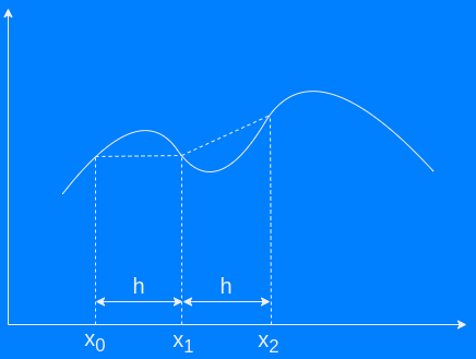
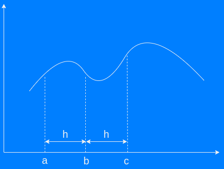
Simpson's 1st rule (1-4-1 rule)

The most used one at least by me is Simpson's 1^st rule also known as Simpson's 1-4-1 rule. It used quadratic interpolation as it is a simplified version of Simpson's 1/3 rule. The length of each interval or distance between each x shall be equal for the simplification to be valid

\begin{align} Area = \frac{h}{3}(a+4b+c) \end{align}

where:

h width between each coordinate i.e. distance between a and b or b and c
a is the y-coordinate at the start of the interval
b is the y-coordinate at the middle of the interval
c is the y-coordinate at the end of the interval

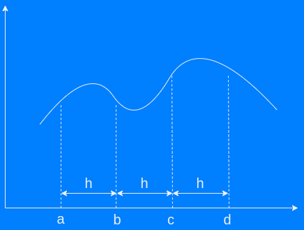
Simpson's 2nd rule (1-3-3-1 rule)

Simpson's 2^nd rule also known as 1-3-3-1 rule is based on Simpson's 3/8 rule and consequently uses quadratic interpolation. Otherwise it is similar to Simpson's 1^st rule although an additional point for each interval is needed.

\begin{align} Area = \frac{3h}{8}(a+3b+3c+d) \end{align}

h width between each coordinate i.e. distance between a and b or b and c
a is the y-coordinate at the start of the interval
b is the y-coordinate located 1/3 of the way from a towards d
c is the y-coordinate located 2/3 of the way from a towards d
d is the y-coordinate at the end of the interval

Simpson's 3rd rule (5-8-1 rule)

The final simplified rule by Simpson is Simpson's 3rd rule also known as 5-8-1 rule.

\begin{align} Area = \frac{h}{12}(5a+8b-c) \end{align}

where:

h width between each coordinate i.e. distance between a and b or b and c
a is the y-coordinate at the start of the interval
b is the y-coordinate at the middle of the interval
c is the y-coordinate at the end of the interval

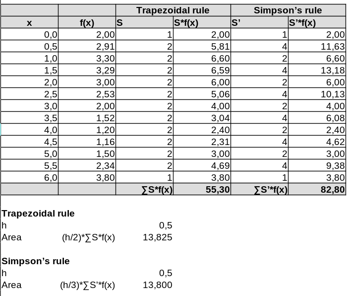
Practical way to determine the area below the curve using Excel or similar

The picture below show one approach to calculate the area below a curve using a spreadsheet like Excel or similar. Two methods are used. The trapezoidal rule and Simpsons's rule. S is the same vector as described in the section showing how to implement the trapezoidal rule in Python. Note the number of x-coordinates i.e. an odd number giving an even number of intervals and the even spacing between them. Both methods requires even spacing between each x when implemented as show here but only the Simpson's rule require an odd number of points and consequently and even number of intervals.

This example uses Simpson's 1st rule (1-4-1 rule) as described above i.e.

\begin{align} Area = \frac{h}{3}(a+4b+c) \end{align}

Hence the vector S' can be determined to following using the same approach as the one used for the trapezoidal rule.

\begin{align} \boldsymbol{S'}=\begin{bmatrix} 1 \cr 4 \cr 2 \cr \vdots \cr 2 \cr 1 \end{bmatrix} \end{align}

Using this the area below the curve can be calculated in a spreadsheet as in the example below.

Determine the area below the curve in Excel or similar using the trapezoidal and Simpson's rule

Using Python

Python has packages that enables numerical integration. My favorite is the package SciPy that contains the modules integrate with among others has implemented the functions simpson and trapezoid. The simple example below show how both of the functions are used. Using the same input as in the spreadsheet example it is seen that the result is the same when using the the functions in SciPy integrate.


# Import of required packages i.e. NumPy for the array
import numpy as np
# Only imports the functions simpson and trapezoid from SciPy.integrate
from scipy.integrate import simpson, trapezoid

# The arrays containing the x and y-coordinates
x = np.linspace(0,6,13)
y = np.array([2,
              2.91,
              3.30,
              3.29,
              3.0,
              2.53,
              2.0,
              1.52,
              1.2,
              1.16,
              1.5,
              2.34,
              3.8])

# Integrate using Simpson's rule
aSimp = simpson(y, x=x)
print("Result using Simpson's rule = ", np.round(aSimp,3))
# Result using the trapezoidal rule =  13.825

# Integrate using the trapezoidal rule
aTrap = trapezoid(y, x=x)
print("Result using the trapezoidal rule = ", np.round(aTrap,3))

# Output will be 
# Result using the trapezoidal rule =  13.825
# Result using Simpson's rule =  13.8

SciPy.integrate contains several functions for numerical integration and also some that are more advanced than the ones shown in this article. For more details I will recommended the documentation for the SciPy integrate module.