Straight line and polynomial equation

It is quite often beneficial to be able to determine the equation of a polynomial going through known points (coordinates). This article will describe the procedure of determining a straight line going through two predefined points and afterwards a polynomial going through 3 or more points by solving the system of linear equations.

Lets start with the most simple case where a straight line going though two points are determined.

Straight line between two known point s

First lets define the equation for a straight line:

\begin{align} y=ax+b \end{align}

where a is the slope or gradient of the straight line and b is the interception with the y-axis i.e. at x=0. The letters used for the two constants for slope and interception varies from country to country and person to person. I have for intance often seen that m is used for slope instead of a . In the following however a will be used as the slope as this is common practice where I live.

Determining the slope a

The equation has two constants (a and b) which has to be determined i.e. two unknowns. Using the two known points (x₁,y₁) and (x₂,y₂) the two equations required to determine a and b can be written as:

\begin{align} y_1=ax_1+b\\ y_2=ax_2+b \end{align}

Solving the equations can be done in multiple ways but here we will solve it by setting b from equation 1 equal b from equation 2 and isolate a.

\begin{align} b=y_1-ax_1\\ b=y_2-ax_2\\ y_1-ax_1=y_2-ax_2\\ \text{Solving for a}\\ a=\frac{y_2-y_1}{x_2-x_1} \end{align}

Determining the interception b

The determined slope a is inserted into \( b=y_1-ax_1 \) or \( b=y_2-ax_2 \) and the constant b is determined. The result will be the same regardless of which point is used.

Example determining the equation for a straight line going through two points

In this example we are going to determine the equation for a straight line by using the coordinates for two points on the straight line. The equation for a straight line is as described in the previous section \( y=ax+b \) hence we need to determine the constants a and b.

The coordinates for the two points are: - Point 1: (2,8) - Point 2: (5,14)

First step is to determine the slope a by using the equation from above

\begin{align} a=\frac{y_2-y_1}{x_2-x_1}=\frac{14-8}{5-2}=2 \end{align}

With the slope a known the interception with the y-axis b can be determined.

Either points can be used to determine b. I have used point 1

\begin{align} b=y_1-ax_1=8-2*2=4 \end{align}

As both the slope a and the interception with y-axis b is know the equation for the straight line going through the two points can be written as:

\begin{align} y=2x+4 \end{align}

Polynomial through points

The complexity of the task increases when the number of points and consequently the degree og the polynomial increases.

The number of known points are important when determining the equation as N number of points give a N-1 degree polynomial leading to N number of unknowns and consequently N number of equations to be solved. As seen the in previous section two points gave a straight line i.e. first degree. Three points will give a second degree polynomial and so forth.

The following will look into the solution for a polynomial going through three known points. The procedure is the same regardless of the number of points but the complexity is somewhat simpler.

The equation for a second degree polynomial is:

\begin{align} y = ax^2+bx+c \end{align}

The constants a, b and c shall be determined. This give 3 unknowns which always requires 3 equations and consequently the coordinates for 3 points are needed.

Point 1: (x₁, y₁)
Point 2: (x₂, y₂)
Point 3: (x₃, y₃)

The three equations needed to determine the constants are defined

\begin{align} y_1 = ax_1^2+bx_1+c\\ y_2 = ax_2^2+bx_2+c\\ y_3 = ax_3^2+bx_3+c\\ \end{align}

This is solved by solving the Linear System

\begin{align} \boldsymbol{Ax}=\boldsymbol{b} \end{align}

First the system of linear equations will be defined as a vector equation before making the matrix to make it clearer how to do it. This extra step is however not needed.

A typical system of equations has the following form:

\begin{align} a_{11}x_1+a_{12}x_2+...+a_{1n}x_n &=b_1 \\ a_{21}x_1+a_{22}x_2+...+a_{2n}x_n &=b_1 \\ & \vdots \\ a_{m1}x_1+a_{m2}x_2+...+a_{mn}x_n &=b_m \end{align}

where \( x_1, x_2, ..., x_n \) are the unknowns.

This can also be written as a vector equation

\begin{align} x_1\begin{bmatrix} a_{11} \cr a_{21} \cr \vdots \cr a_{m1} \end{bmatrix} +x_2\begin{bmatrix} a_{12} \cr a_{22} \cr \vdots \cr a_{m2} \end{bmatrix}+...+ x_n\begin{bmatrix} a_{1n} \cr a_{2n} \cr \vdots \cr a_{mn} \end{bmatrix}= \begin{bmatrix} b_{1} \cr b_{2} \cr \vdots \cr b_{m} \end{bmatrix} \end{align}

The column column vectors a can be transformed into a matrix A. Hence we now have a typical system of linear equations.

\begin{align} \left[ \begin{matrix} a_{11} & a_{12} & \cdots & a_{1n} \cr a_{21} & a_{22} & \cdots & a_{2n} \cr \vdots & \vdots & \ddots & \vdots \cr a_{m1} & a_{m2} & \cdots & a_{mn} \cr \end{matrix} \right] \begin{bmatrix} x_{1} \cr x_{2} \cr \vdots \cr x_{n} \end{bmatrix}=\begin{bmatrix} b_{1} \cr b_{2} \cr \vdots \cr b_{m} \end{bmatrix} \end{align}

The next step to determine the polynomial going through the known points is it setup the matrix A and the column vector b for this specific case. One important note is that in the matrix form shown above x is the unknowns and A and b is the known. This is contrary to the first three equations.

\begin{align} y_1 = ax_1^2+bx_1+c \\ y_2 = ax_2^2+bx_2+c \\ y_3 = ax_3^2+bx_3+c \\ \end{align}

From this it can be seen that the column vector b is

\begin{align} b=\begin{bmatrix} y_{1} \cr y_{2} \cr y_{3} \end{bmatrix} \end{align}

The column vector with the unknowns x is:

\begin{align} x=\begin{bmatrix} a \cr b \cr c \end{bmatrix} \end{align}

and the matrix A is defined as

\begin{align} A=\left[ \begin{matrix} x_1^2 & x_1 & 1 \cr x_2^2 & x_2 & 1 \cr x_3^2 & x_3 & 1 \end{matrix} \right] \\\end{align}

The system of linear equations can be solved by hand but is much more easily solved by using python.

Solving the System of linear equations using Python and numpy

Using python and the package NumPy is an easy way to solve a system of linear equations. As a side note. My preferred way to install python and NumPy is to use the freely available Anaconda Distribution.

Below is python script used to solve the system of linear equations.


# Import required package. In this case only numpy
import numpy as np

# Define the coordinates for the three known points
x1 = -2
y1 = 3

x2 = 2
y2 = 7

x3 = 3
y3 = 18

# Solve the system of linear equations Ax=b by using numpy
A = np.array([[x1**2, x1, 1], [x2**2, x2, 1], [x3**2, x3, 1]])
b = np.array([y1, y2, y3])
x = np.linalg.solve(A,b)

# Print the result
print(x)

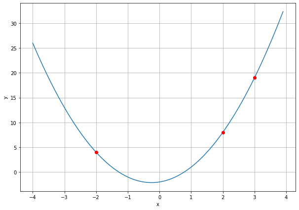
The result output in the console is: [ 2. 1. -3.] hence a=2, b=1 and c=-3 and writing the complete equation for the polynomial going through the three points.

\begin{align} y = 2x^2+x-3 \end{align}

The final check is to plot the points and polynomial to ensure that the result is correct.