Interpolation
Interpolation is an important topic as it enables us to find intermediate values between known values e.g. when finding thermodynamic properties in a table.
Several methods of interpolation exists with difference complexity and accuracy. In this article we will only look at a couple of the methods. The first is linear interpolation as this is most likely the most used one due to simplicity. It can easily be done by hand and be implement in a spreadsheet. Secondly we will briefly look at polynomial and spline interpolation and finally show examples on how to interpolate using a spreadsheet (Microsoft Excel, LibreOffice Calc, Google Sheet etc.) and Python for the more advanced methods.
Linear interpolation
Linear interpolation is maybe the most used method for interpolating values between known data points. The reason being is simplicity as it only uses the two nearest data points and assume a straight line between them.
Interpolating the y-value at the target x which lie between xa and xb is simply calculated using the equation below.
where - x is the x-value at which y shall be determined at - (xa, ya) is the first known data point xa<=x - (xb, yb) is the second known data point xb<=x
It is important to choose data points on either sides of the x-value and as close as possible to the value of x to obtain a valid and accurate result.
Polynomial Interpolation
Polynomial interpolation can in some cases be more precise than linear interpolation. It is however not as simple nor as quick as the equation for the polynomial will have to be determined. The degree of the polynomial will depend upon the number of known data points as N number of data points will lead to N-1 degree polynomial. Using only two points will lead to a straight line i.e. the same result a linear interpolate hence three or more points are needed.
This website already contains a more detailed article describing how to determine a polynomial going though N number of data points. See more here.
With the equation for the polynomial determined the y value for the target x can be determine by entering the x value into the equation.
It is in my point of view important to plot the polynomial together with with the data points to determine if the result is valid. The reason being that higher order polynomials determined this way can suffer from Runge's Phenomenon meaning that it will oscillate between the data points and not be valid.
Spline interpolation
Splines originally originates from the elastic rulers used by Naval Architects to make faired hull lines.
Spline interpolation is similar to polynomial interpolation. The difference is that instead of fitting one high degree polynomial through all points one can instead use lower degree piecewise polynomials. It solves the challenge with Runge's Phenomenon.
Spline interpolation is very cumbersome by hand and it is even in Excel quite difficult to implement. My preferred way to do spline interpolation is to use our own Interpolation Calculator or Python as described in one of the following sections.
How to use the Interpolation Calculator
The simplest way to interpolate between two data points or a complete series of data poitns is to use the calculator in this website. It requires two or more data points and can do linear, polynomial and cubic (3rd order) spline interpolation. It will for the first two methods also output the interpolation functions. Further it calculates the y-value at a specific x if entered and plot each of the of the interpolation functions making it easy to select the best one for the specific use case.
How to interpolate using Excel or similar software
Interpolation can be carried out in a spreadsheet like Microsoft Excel, LibreOffice Calc and Google Sheet. Linear interpolation is relatively simple but other interpolation methods are quite difficult to implement in Excel without writing macros in VBA or similar. Only linear interpolation will be dealt with in the following.
Two data points
In the simplest case only two data points is used.
The figure below show a simple linear interpolation calculator. It works by entering the coordinates for data point 1 and 2.
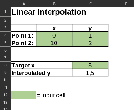
It works by inputting the known data points in the table i.e. the first four green cells. Secondly the target x value shall be added. This shall be between the two x values written in the table. Finally we can now calculate the y-value at the target x.
In cell C9 the equation for linear interpolation (see section Linear Interpolation above)
=+C4+(C5-C4)*(C8-B4)/(B5-B4)
A complete series of data points
The above example only contains two points but often one will have a complete series of data points. Normally the two data points closest to the target x i.e. one on each side is selected from the series of data points and the normal procedure using linear interpolation is used as described above. It is also possible make a spreadsheet in either Excel, Google Sheet or LibreOffice Calc where the complete series of data is entered and linear interpolation used.
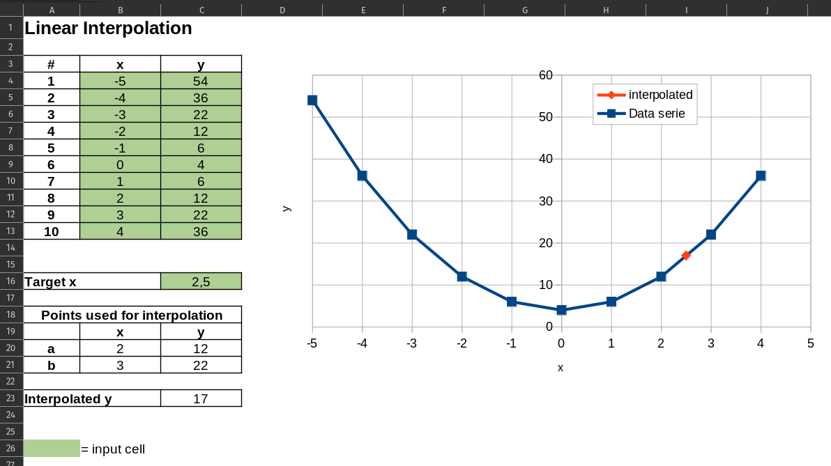
Having a series of data points instead of just two requires an extra step. If we were to do this by hand we would first determine the x-values closest to the target x with one being smaller and the other larger.
The same shall be done when doing this in a spreadsheet. This can be done using the functions index and match. The match function searches for a given value in a range of cells. It can either search for the exact value or the largest value that is less than or equal to or the smallest value that is more than or equal to the given value and returns a relative position.
MATCH(lookup value;search range;type)
The match takes three inputs:
- Lookup value is the value to be found. In this case the target x
- Search range is the range of cells to be searched. The relative position returned by the match function relates to the range i.e. position 1 is the the first cell and so forth.
- Type can either be set to -1, 0 or 1. 0 is used if the exact match is needed. -1 and 1 is for when the a value smaller or larger than the lookup value shall be found when an exact match is not found. In this case we use 1 or we want to find a value smaller than or equal to the lookup value and the the values in the search range is decending.
The match function will look like this:
MATCH($C$16;$B$4:$B$13;1)
Using the match function alone only gives us the relative position of the value but what is needed to the actual value. To determine the value the index function is used.
INDEX(array, row_num, [column_num])
The index function takes three inputs
- array the cell range containing the data
- row_num the selected row number relative the the chosen cell range
- column_num is optional. Column number relative to the chosen cell range
Combining the two will lead to a function lookin like this in cell B20
INDEX($B$4:$C$13;MATCH($C$16;$B$4:$B$13;1);1)
where the match function is used to determine the row number and the index function returns the value.
The formula in cell C20 is very similar. Only difference being that the column_num is changed from 1 to 2 as the y value is needed.
The formulas in B21 and C21 is very similar to the formulas in row 20. The difference being that now the next value in the dataset is required hence we add 1 to the match function MATCH($C$16;$B$4:$B$13;1)+1
Cell B21
INDEX($B$4:$C$13;MATCH($C$16;$B$4:$B$13;1)+1;1)
Cell C21
INDEX($B$4:$C$13;MATCH($C$16;$B$4:$B$13;1)+1;2)
The final step is to use linear interpolation between the two selected points using the same procedure as in the example having only two points.
Cell C23 will then be
C20+(C21-C20)*(C16-B20)/(B21-B20)
Interpolation using Python, Numpy and SciPy
A different approach is to use Python and the packages NumPy and SciPy. This can be an advantage when having large amount of data or if using more advanced interpolation methods.
Both NumPy and SciPy contains routines for interpolation. NumPy has a function numpy.interp for one-dimensional linear interpolation. I will however use scipy.interpolate.interp1d instead in this example as it functions quite similarly but allows for different types of interpolation methods.
The first step is to load the needed packages. The needed packages are NumPy for the array function to store the data points and interpolation is needed from the package SciPy. As an option matplotlib.pyplot can be imported for plotting purposes.
import matplotlib.pyplot as plt
import numpy as np
from scipy import interpolate
Next step is to enter the data points into the NumPy arrays
x = np.array([-5,-3,-1,1,3,4])
y = np.array([54,22,6,6,22,36])
The interpolation functions is created using SciPy interp1d.
fLinear = interpolate.interp1d(x,y,kind='linear')
fCubic = interpolate.interp1d(x,y,kind='cubic')
The interp1d function has several options depending on its use case. In its simplest form it takes two inputs i.e. x and y. In the example above kind has been added as well. It allows control over the type of interpolation used e.g. kind='linear' for linear and kind='cubic' for third order spline interpolation.
The final step is to determine the y-value at the target x.
xTarget=2.5
print("Linear interpolation           y = ", fLinear(xTarget))
print("3rd order spline interpolation y = ", fCubic(xTarget))
Combining it all the script for interpolation in Python will end up looking like this.
import numpy as np
from scipy import interpolate

x = np.array([-5,-3,-1,1,3,4])
y = np.array([54,22,6,6,22,36])

x1 = np.linspace(np.min(x),np.max(x),200)

fLinear = interpolate.interp1d(x,y,kind='linear')
fCubic = interpolate.interp1d(x,y,kind='cubic')

xTarget=2.5
print("Linear interpolation           y = ", fLinear(xTarget))
print("3rd order spline interpolation y = ", fCubic(xTarget))
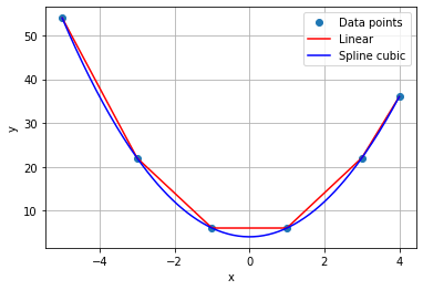
Plots like the one above can be made using Matplotlib. Below is the python code used to make the plot above
x1 = np.linspace(np.min(x),np.max(x),200)

plt.plot(x,y,'o')
plt.plot(x1,fLinear(x1),'-r')
plt.plot(x1,fCubic(x1),'-b')

plt.grid(True)
plt.xlabel('x')
plt.ylabel('y')
plt.legend(['Data points','Linear','Spline cubic'])